
A financial organizations may commonly face one question: I have a certain projected amount of cashflow needs in the future, and I have a bunch of bonds I can invest, how should I choose the individual securities to best meet my cashflow needs? Of course part of this question falls into the scope of fundamental research to select the security in the appropriate sector/rating, but this question can also be partly solved using quantitative method by leveraging on Linear Programming.
A general linear programming problem can be stated as the form as follows:
There are two important characteristics of the linear programming:
- The first one is the objective function should be a linear combination of the decision variables (x)
- The second one is the feasible region, by design, is a convex set. This is because each individual linear constraint forms a convex set and the feasible region is hence an intersection of convex sets, which are also convex. [A set S is said to be convex if for any two points in S, all their linear combinations are also in S]
To show the second point, please refer to the following graph which gives a graphic representation of the convex set and how intersection works.

The great property of this problem is that for a convex feasible set, the linear objective must reach an optimum (min or max) at at least on vertex. Therefore, to find the optimal solution, it suffices to just check all the vertices, which creates a simple and robust optimization method called simplex method.
Next, let’s see how we can formulate the problem mentioned at the beginning of this article to linear programming. Let’s consider there is a portfolio of n bonds to choose from, and each bond there is a cashflow for each time, hence creating a n by m matrix of cashflow (the F matrix below).
The decision variable (x) is how many bonds should be purchased for each bond, with the constraint of the cashflows from all bonds is greater than the required liability cashflow (the L matrix below) for each time period.
The objective is to minimize the total cost of the portfolio. Hence, the question can be formulated as:
However, this formulation is restrictive as it asks the cashflow generated in each period only is sufficient to cover the liability. However, if short-term bonds are more attractive, it is possible that more short-term bonds should be purchased and the surplus in previous periods can also be used to offset later laibility cashflows. To formulate this, additional surplus variables are created. Also, it should be noted that with these surplus varibles introduced, to minimize the cost the constraints should natuarally be tight (i.e. the bond cashflow plus surplus should just be able to match the liability cashflow. There is no excess needed. ) Hence, the problem can be formulated as:
Or in matrix notation:
Where R is in the form of:
With the problem formulation ready, some potential bond portfolio and liability constraints, as well as a dummy discount rate are randomly created to show how it works. The inputs are as follows:
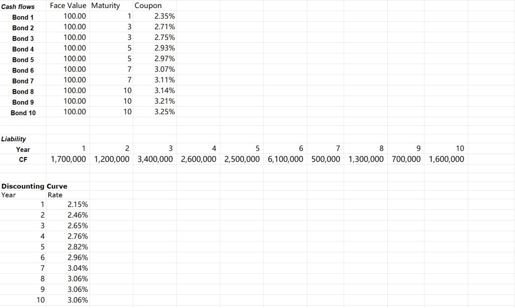
The dummy bond portfolio and discount curves are as above. With that, two sets of bond prices are tested. In the first set, every bond is discounted with the same discount curve (the dummy curve supplied), so all bonds of the same maturity are essentially equivalent. Some bonds are purposedly made traded at discount in the second set, and the optimization then should choose these bonds with higher yield if correct. The optimization result is as above. The python cvxpy package is used in formulating and solving the linear programming problem.
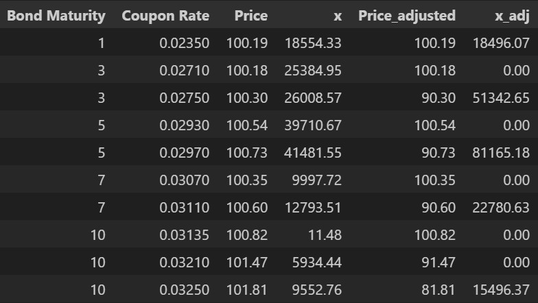
From the result, while for the first set of bond prices, the optimizer allocates more or less evenly across the bonds with the same maturity as they are equivalent and optimizer cannot distinguish them too much, for the second set the optimizer does allocate to the bond with highest yield as expected.
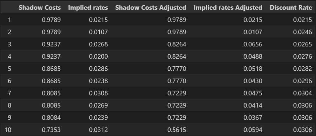
Also, in addition to the optimization result itself, there is another interesting result that come naturally with the optimization – the so-called shadowed cost. This is defined as what is the increase in the objective (cost for purchasing bond) with an additional unit increase in each of the constraint (liability cashflow). In this optimization problem, it naturally interesting because this can be compared to the implied zero-coupon bond price / discount rate from the bond portfolio, as price of the additional unit increase in time t at time 0 is naturally a ZCB maturing at time t.
However, it should be noted that this implied discounting rate is a discount rate that is achievable from the given bond portfolio and hence may not conform with the actual discount rate. From the result below, it can be seen that while the t=1 implied rate exactly matches, as we have exactly one bond in the portfolio maturing in t=1 that follows the market discount rate, the discount rate afterwards are naturally not the same. This comparison can also be used to evaluate the bond portfolio against the market.
Hopefully, after reading this post, you can have a better idea of how quantitative method can be used in selecting the bonds that best satisfy your cashflow needs. As always, feel free to contact me or leave a comment for any question you have or any interesting topic that you want to explore in your mind!

Leave a comment