BZ Consulting LLC

“Good afternoon, everyone” has been driving the market crazy for quite some time. The Fed decision directly affects the federal funds rate which then spread its impact towards market rates like treasury yield. In this post, we try to understand how this mechanism works, and more generally when we talk interest rate movement, how do we view it and what’s the associated risk.

How Fed decision translates to interest rate movement

Let’s take a closer look at how each fed decision translate into market movement. The FOMC adjust the target range of the federal fund rate, which is the interest rate charged by banks to borrow from each other over night. The Fed maintains the effecitve fed fund rate within the range it sets via various tools:

• Interest on Reserve Balance: This is the interest paid on funds that banks hold in their reserve balance accounts at their Federal Reserve bank. As Banks can always earn this rate, they would be better off holding the reserve than lending out money with a rate lower than this interest. Therefore, it can serve as a floor for the lending rates of the banks.

• Overnight Reverse Repurchase Agreement: For financial institutes that cannot earn interest on reserve balance, the reverse repo also serves as a way for these financial institutes to earn rate from the Fed. This is a supplement tool to put a floor on the lending rates in the market.

• Discount Rate: This is the rate the Fed charge for loans it makes. As banks are not likely to borrow fund from others at a higher rate if they can borrow from the Fed at this rate, this discount rate sets a ceiling for the fed fund rate.

Therefore, we can see that by changing the fed fund rate target, it can translate the impact into market rate movement via the following:

The fed fund rate affects the banks’ short term funding rate, which then move the short term funding rates like repo rates in general financial markets. Therefore, the short term treasury yields will move as if I can only borrow from repo at 5%, it is likely one will ask for a higher yield to compensate for the borrowing cost. This impact is market mechanical.

Then the expectation come into play, where if the market anticipates there are more hikes to come, then the future short rate shall also increase and this translate to long term yield change. However, if it is towards the end of rate hike cycle and market does not anticipate further rate hikes, the long end might not move up much.

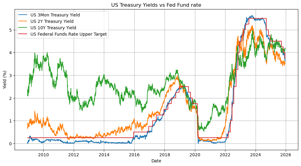
However, it should be noted that the treasury yields are still determined via supply and demand. The yields are of course moved by other longer term expectations on business and growth, other demands like foreign investment, collateral demand etc. It can be seen from the graph below that while the 3 Mon curve tracks the fed fund rate more closely as there is more market mechanical effect, there are more uncertainties the longer the yield curve extends.

Let’s take a closer look at how each fed decision translate into market movement. The FOMC adjust the target range of the federal fund rate, which is the interest rate charged by banks to borrow from each other over night. The Fed maintains the effecitve fed fund rate within the range it sets via various tools:

Interest on Reserve Balance: This is the interest paid on funds that banks hold in their reserve balance accounts at their Federal Reserve bank. As Banks can always earn this rate, they would be better off holding the reserve than lending out money with a rate lower than this interest. Therefore, it can serve as a floor for the lending rates of the banks.

Overnight Reverse Repurchase Agreement: For financial institutes that cannot earn interest on reserve balance, the reverse repo also serves as a way for these financial institutes to earn rate from the Fed. This is a supplement tool to put a floor on the lending rates in the market.

Discount Rate: This is the rate the Fed charge for loans it makes. As banks are not likely to borrow fund from others at a higher rate if they can borrow from the Fed at this rate, this discount rate sets a ceiling for the fed fund rate.

Therefore, we can see that by changing the fed fund rate target, it can translate the impact into market rate movement via the following:

The fed fund rate affects the banks’ short term funding rate, which then move the short term funding rates like repo rates in general financial markets. Therefore, the short term treasury yields will move as if I can only borrow from repo at 5%, it is likely one will ask for a higher yield to compensate for the borrowing cost. This impact is market mechanical.

Then the expectation come into play, where if the market anticipate there are more hikes to come, then the future short rate shall also increase and this translate to long term yield change. However, if it is towards the end of rate hike cycle and market does not anticipate further rate hikes, the long end might not move up much.

However, it should be noted that the treasury yields are still determined via supply and demand. The yield are of course moved by other longer term expecations on business and growth, other demands like foreign investment, collateral demand etc. It can be seen from the graph below that while the 3 Mon curve tracks the fed fund rate more closely as there is more market mechanical effect, there are more uncertainties the longer the yield curve extends.

How interest rate curve generally moves

So, it can be seen that differnt maturities on the yield curve can react differently to fed fund rate change, and in fact their movement is generally different on any day. Given there are so many maturities on a single yield curve and the yield curve moves constantly, it would be then interesting to see if there’s any underlying pattern and if the seemingly random movement can be decomposed to a small number of patterns, then we can manage these patterns to harvest gain / control risk.

Luckily, the interest rate movement can indeed be decomposed to 3 major movement structures. This can be done via Principal Component Analysis (PCA), which is a dimension reduction technique. The idea is simple, the yield curve movement is the joint movement of different points (maturities) on the curve, and this constructs a high-dimensional (different points) movement. PCA decomposes this to a series of linear combination of the individual points movement and the major joint movements (identified by how much variance of movement this linear combination can explain) can be identified.

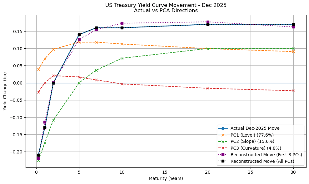
The treasury data from Jan. 2000 to Dec. 2025 are used to construct our PCA analysis to identify the general pattern. Then, Jan. 2025 and Dec. 2025 are chosen as an example to demonstrate how PCA helps to explain the month-to-month rate movement.

From both graphs, it can be seen that while retaining all principal components will exactly reconstruct the graph, retaining only the top 3 can already provide a quite good estimation. It should be noted that as this post focus on introduction and historical risk decomposition, there is no separation between train and test and hence the perfect reconstruction is achievable. Depending on the detailed application, the separation may become necessary, but PCA shall still achieve a quite satisfactory result.

Over all sample period, the first three components explained ~95% of the variance of the interest rate movement. The first component features a relatively flat shape across all maturties and is thus called a “level” component. The second component features a contrust between the far-term and near-term maturies, and hence called “slope” component. Finally, the third component features the contrast between the two ends and the belly, and is thus called the “curvature” component.

Apart from the statistical power, there are also good reasons to associate with each component movement. The level movement is more linked to long term expectation that will affect all times, like persistent growth/recession and inflation, and the risk premia, much of them inferred from the monetary policy. The slope movement, on the other hand, demonstrates the expectation on different behavior across time, like if there is a recession expectation then the future rates will probably drop significantly, leading to the far-end of the rates drop while the current rate remains temporary high as current target rate has not been cut yet. The curvature movement can be more tied to liquidity as there are strong 5–7-year treasury issuance and the demand and supply will drive the belly part of the curve strongly

Application on Risk Management

Now that the movement can be more neatly summarized and explained, how can it help in risk management? When managing interest rate risk, it is desired to understand how much risk (i.e. market value loss of portfolio ) when the rate increases. While duration provides a good estimation of market value movement for parallel shift, it can be seen that the rate movement is not always parallel.

A common way to quantify the risk is by revaluating the bond portfolio under a shock scenario under which the rates do not only move parallelly, but the challenge for rates is how to define a shock quantitatively as the curve is composed of so many spot rates. This is when the PCA component analysis introduced above becomes very handy as for each component, it a create a univariate score for a whole curve, and thus shock scenario under each curve can be created by ranking now easily. Also, as each component in PCA is orthogonal to each other, the risk can also be aggregated easily.

Feel free to shoot an email to ask if you have any question after reading the post / want any quantitative demo. Also leave a message if you have any interested topic desired to learn. Happy New Year!